AIAS+ 2026
The research talk explains conditional generation, precipitation constraints, and the difference between a valid field and a useful downscaled field.
Conditional field generation meets checkable precipitation constraints and a measured PyTorch export and serving path.
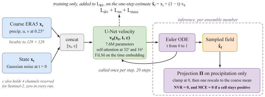
PC-RF studies how a generative downscaler can produce conditional fields while keeping its output constraints explicit. The model learns a rectified-flow velocity field. The sampler integrates that field from Gaussian noise, then applies a precipitation operator that clamps negative values and matches a coarse mean.
The project also exports the velocity network into AOTInductor and ONNX artifacts. Python and Rust samplers keep the integration loop and output checks outside the network graph. The measured engineering results cover backend timing, numerical parity, and a corrected distributed-training sweep.
The output checks establish nonnegative precipitation and agreement with a supplied coarse mean under the operator's stated conditions. They do not establish accurate rain placement, calibrated uncertainty, or useful climate downscaling. The historical climate comparison is superseded, and the page makes no current claim that the soft penalties improve climate skill.
The AOTInductor full-sample median uses random weights on an A100.
The corrected four-worker sweep measures synthetic training throughput.
The benchmark uses the recorded ERA5 network architecture.
The A100 benchmark JSON records the timing and parameter count. The DDP-correct CSV records the training rate. Both records are explained below.
The two recordings explain different parts of the same research-engineering project.
The research talk explains conditional generation, precipitation constraints, and the difference between a valid field and a useful downscaled field.
The engineering talk follows the model through export, numerical checks, serving runtimes, and the distributed-training bug that invalidated an earlier scaling curve.
The recordings and PDFs preserve their conference versions, including earlier climate figures. The later evaluation audit on this page supersedes those scientific result claims. The public materials repository contains talk assets and does not release the private implementation.
A coarse field supplies the large-scale context, while a conditional generator samples possible fine fields. The coarse precipitation mean also supplies the value that the output contract must preserve.
| Part | The conference implementation uses the following definition. |
|---|---|
| Input | The model receives coarse precipitation and horizontal wind, an upsampled conditioning tensor, a sampled noisy state, and flow time. |
| Output | The sampler returns a fine-grid precipitation and wind tensor. Multiple noise draws give an ensemble. |
| Learning objective | The network fits the noise-to-reference displacement and optionally adds soft penalties on a clean-field estimate. |
| Hard output constraints | The precipitation channel must be nonnegative, and its domain mean must equal the supplied coarse mean. |
| Diagnostic | The wind derivative term is a soft diagnostic. It is not an output certificate. |
| Scientific objective | A valid evaluation must also measure fine-scale predictive skill against an independent, time-aligned reference. |
The recorded architecture operates on a three-channel \(128\times128\) field and seven conditioning channels. The condition contains upsampled precipitation, upsampled wind components, and four zero-filled slots. The conference experiments used no Sentinel-2 information.
The architecture record names src/pcrf/model.py, src/pcrf/data.py, and the conference numbers ledger as its sources.
The training procedure samples a reference field \(x_1\), Gaussian noise \(x_0\), and a time \(t\). It places the training state on the straight segment between the noise and reference.
\[x_t=(1-t)x_0+t x_1,\qquad t\sim\mathcal U(0,1),\qquad x_0\sim\mathcal N(0,I).\]
The displacement \(x_1-x_0\) supplies the supervised target. The conditional network predicts that displacement from the intermediate state, time, and coarse condition \(c\).
\[\mathcal L_{\mathrm{RF}}=\mathbb E\left[\left\|v_\theta(x_t,t,c)-(x_1-x_0)\right\|^2\right].\]
The quantity \(v_\theta\) is a rate of change in the generated tensor. It is not atmospheric wind. The generated wind channels are values inside that tensor.
The equations follow src/pcrf/flow.py and the rectified-flow construction of Liu, Gong, and Liu.
The velocity network concatenates \(x_t\) and the coarse condition before its input convolution. Residual blocks and skip connections carry features across the U-Net. A sinusoidal time embedding enters the residual blocks, and time-only FiLM modulates the first feature map.
The recorded model uses resolution levels \(128,64,32\) above a \(16\times16\) bottleneck. Self-attention runs at the \(32\times32\) level and in the bottleneck. The benchmark architecture contains 7,565,251 parameters.
The model record and benchmark configuration source these dimensions. The conditioning path uses concatenation, and the attention is self-attention.
The sampler starts from new Gaussian noise and advances the state through forward Euler steps. The conference configuration uses 20 steps.
\[x_{k+1}=x_k+\Delta t\,v_\theta(x_k,t_k,c),\qquad \Delta t=\frac1K,\qquad K=20.\]
The final precipitation projection acts after the integration loop. The sampler can draw several members from the same coarse condition by changing the initial noise.
The benchmark configuration records the step count. The conference implementation records the loop in src/pcrf/flow.py.
The physics terms act on a one-step estimate of the clean field. The estimate extends the current velocity to the end of the interpolation interval.
\[\widetilde x_1=x_t+(1-t)v_\theta(x_t,t,c).\]
The original training objective adds negative-precipitation, domain-mean, and wind-derivative penalties to the flow loss.
\[\mathcal L=\mathcal L_{\mathrm{RF}}+\lambda_{\mathrm{nn}}\mathcal L_{\mathrm{nn}}+\lambda_{\mathrm{mass}}\mathcal L_{\mathrm{mass}}+\lambda_{\mathrm{wind}}\mathcal L_{\mathrm{wind}}.\]
\[\mathcal L_{\mathrm{nn}}=\mathbb E\left[\|\min(\widetilde p,0)\|^2\right],\qquad\mathcal L_{\mathrm{mass}}=\mathbb E\left[(\operatorname{mean}(\widetilde p)-m_c)^2\right].\]
The intended wind term penalizes squared horizontal divergence. The historical ERA5 array order and channel scaling prevented that calculation from representing physical divergence. The later audit supersedes the old derivative results, and the new study drops that penalty.
A penalty changes the training objective, but it does not make the output satisfy a hard constraint. The recorded climate experiments show no established benefit from the penalties. The terminal operator provides the two precipitation guarantees under its stated conditions.
The released paper documents the original loss. The scope record follows the later research audit and distinguishes the original formulation from the proposed evaluation.
The operator first replaces negative precipitation with zero. It then multiplies the entire precipitation channel by a scalar that matches the coarse mean.
\[q_i=\max(\widehat p_i,0),\qquad \mu=\frac1n\sum_{i=1}^{n}q_i.\]
\[p_i^*=q_i\frac{m_c}{\mu}\qquad\text{when }\mu>0\text{ and }m_c\ge0.\]
The proof is direct. Each \(q_i\) is nonnegative, and the rescale factor is nonnegative. The new mean equals \(\mu(m_c/\mu)=m_c\). The equality holds up to floating-point rounding in an implementation.
The rescale preserves ratios among positive cells. It cannot place a rain band, restore a missing storm, or repair an incorrect reference. The clamp changes the field where values were negative.
The operator belongs to established work on constrained generation. The page credits Hess et al. and Harder et al. and makes no novelty claim for the global rescale.
An all-clamped field has \(\mu=0\). A positive target mean then makes the division undefined. The conference Python serving copy floors the denominator, while the Rust copy skips rescaling for a sufficiently small clamped mean. Both leave an all-clamped field at zero and fail its positive target.
The conference serving copies also skip rescaling when the target mean is zero. A clamped field that remains wet then fails the dry-target contract. An output gate must check the result rather than assume the runtime enforced that contract.
The legacy serving MCE helper returns zero for sufficiently small targets. That branch can hide the dry-target failure, so an absolute mean-error check is needed.
The newer local research implementation adds a uniform fallback that fills the selected cells with \(m_c\). It also supports masks, area weights, and block constraints. Those changes do not establish that the conference Python and Rust serving runtimes received the same update.
The implementation record separates src/pcrf/physics.py from src/pcrf/serving/math.py and services/inference-rs/src/physics.rs.
The browser computes this illustrative example. The values are chosen for explanation, and they are not measurements from ERA5 or a trained model.
The non-negativity violation rate (NVR) counts negative precipitation cells. The mass-conservation error (MCE) compares the generated mean with the coarse mean.
\[\mathrm{NVR}=\frac1n\sum_i\mathbf1[p_i<0],\qquad \mathrm{MCE}=\frac{|\operatorname{mean}(p)-m_c|}{|m_c|}\quad(m_c>0).\]
A dry target needs an absolute-error check because the relative denominator vanishes. A useful release gate must also check finite values and verify the mean after projection. A constant field can pass the precipitation contract, so the certificate is necessary but insufficient for scientific use.
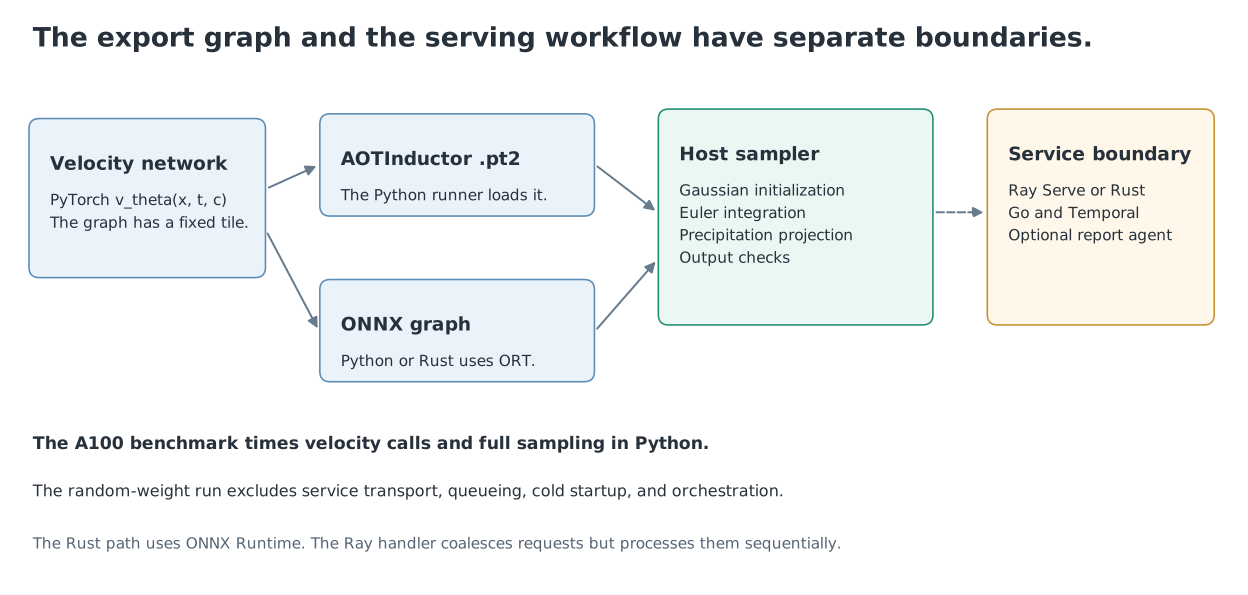
The exporter captures \(v_\theta(x,t,c)\), not a complete request workflow. AOTInductor packages compiled PyTorch execution into a .pt2 artifact. ONNX exports the same network into a graph that ONNX Runtime can execute.
The exported spatial shape stays fixed. The batch dimension is dynamic within its recorded export bound. The integration loop, random-state setup, terminal precipitation projection, and output checks remain runtime responsibilities.
The benchmark compares PyTorch eager, torch.compile, AOTInductor, and ONNX Runtime's CUDA execution provider. The native Rust service uses ONNX Runtime and implements its own sampler and precipitation operator.
The implementation record names export_aoti.py, export_onnx.py, bench_serving.py, and the Rust service. The PyTorch AOTInductor documentation describes the packaging mechanism.
| Layer | The layer owns this work. | The evidence supports this scope. |
|---|---|---|
| PyTorch and Ray Train | The training loop computes the flow loss, synchronizes gradients, and saves training state. | The corrected scaling sweep uses synthetic data on one multi-GPU node. |
| Python and Ray Serve | The serving path loads an artifact and performs sampling and projection. | The recorded CPU smoke verifies the sampler path. The request batch handler processes its coalesced requests sequentially. |
| Rust and ONNX Runtime | The native service executes the velocity graph and its own sampler and output checks. | The recorded smoke tests verify a small demo export. The A100 table times the Python benchmark, not the Rust HTTP service. |
| Go and Temporal | The control-plane design submits and coordinates inference workflows. | The backend timing table excludes this layer. The page makes no production deployment claim. |
| vLLM or SGLang | An optional language model can call the downscaler as a tool and write a report. | The language-model engines belong to the report layer. They do not serve the rectified-flow model itself. |
The runtime scope record identifies the source modules and recorded smoke evidence for each path.
The benchmark uses the recorded ERA5 architecture with random weights because the trained checkpoints were no longer available. It measures execution cost and numerical consistency, and it measures no climate skill.
The recorded device is an NVIDIA A100-SXM4-40GB. The run uses PyTorch 2.14.0+cu130 and ONNX Runtime 1.30.0. The velocity measurement uses 10 warmups and 100 timed calls. The full-sample measurement uses 2 warmups and 30 timed samples. A full sample contains 20 Euler steps and the terminal projection.
The original JSON records the environment, random-weight flag, iteration counts, and all measurements.
| Backend | Velocity p50, batch 1 | Full-sample p50 / p99, batch 1 | Full-sample throughput, batch 32 |
|---|---|---|---|
| PyTorch eager, fp32 | 8.08 ms | 91.7 / 159.8 ms | 45.3 samples/s |
| torch.compile | 2.74 ms | 49.1 / 49.7 ms | 61.6 samples/s |
| AOTInductor | 2.23 ms | 43.3 / 44.2 ms | 61.7 samples/s |
| ONNX Runtime, CUDA EP | 3.37 ms | 65.5 / 66.8 ms | 37.3 samples/s |
The table rounds the recorded measurements using the conference ledger's display precision. Batch-32 throughput uses the mean full-sample time.
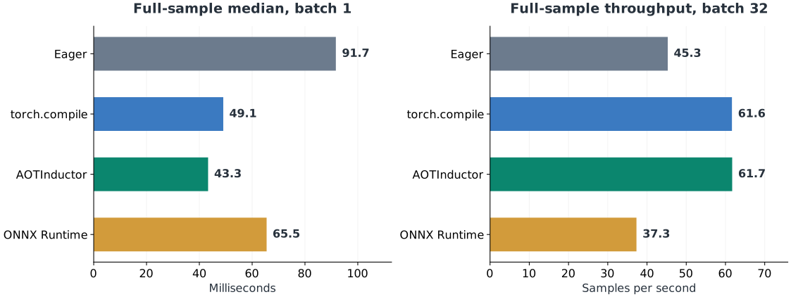
The AOTInductor median is about 2.1 times faster than eager for one full sample in this run. The ratio is \(91.7/43.3\). The timing excludes HTTP transport, queueing, request parsing, cold startup, and the Go or Temporal workflow.
The default PyTorch configuration enables TF32 for cuDNN convolutions and disables it for matrix multiplication. The recorded maximum absolute velocity error is about \(10^{-3}\) for the compiled PyTorch backends and about \(1.5\times10^{-3}\) for ONNX Runtime.
A separate parity-only run disables both PyTorch TF32 switches. The compiled PyTorch errors then fall below \(2\times10^{-6}\). ONNX Runtime remains near \(10^{-3}\), and the PyTorch switch does not control that backend.
The parity comparison covers velocity outputs at batch sizes 1, 4, and 8. It does not establish matched final ensemble distributions or unchanged climate skill. Every timed backend reports zero post-projection NVR on the benchmark inputs. The largest recorded MCE is about \(7.45\times10^{-8}\).
The default benchmark and TF32-disabled parity record support these results. The page makes no claim about the cause of ONNX Runtime's remaining gap.
The earlier training loop wrapped the model in DistributedDataParallel (DDP), then called a custom loss through rf.module. The call bypassed the wrapper's forward path, so the ranks trained independent replicas without the intended gradient synchronization.
The correction adds a RectifiedFlow.forward() that returns the training loss. The loop calls rf(...) through the DDP wrapper. The revised throughput calculation uses the all-reduced sample count and the slowest rank's epoch duration.
# The DDP wrapper receives the forward call.
loss, logs = rf(reference_field, condition, coarse_mean)
loss.backward()
The verified replacement sweep runs on one A100 node with one, two, and four workers. It uses synthetic fields, a \(128\times128\) tile, base width 64, batch 32 per worker, and 40 epochs.
| Workers | Measured samples/s | Derived efficiency |
|---|---|---|
| 1 | 158.0 | 1.00 |
| 2 | 304.8 | 0.96 |
| 4 | 569.4 | 0.90 |
\[\mathrm{efficiency}(W)=\frac{\mathrm{throughput}(W)}{W\,\mathrm{throughput}(1)}.\]
The corrected CSV and sweep configuration record support the table. The values are rounded for display, and the efficiency uses the original CSV values.
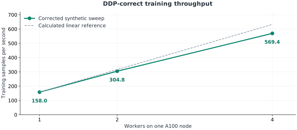
A real two-rank CPU regression check compared gradients on different input data before the replacement GPU run. The corrected measurements support a four-worker synthetic throughput claim. The earlier eight-worker and inter-node curves remain invalid as data-parallel results.
The conference evaluation paired ERA5 coarse precipitation with ERA5-Land precipitation. The audit found problems with the reference, time windows, wind metric, and baseline configuration. The historical quality tables are archival, and the page does not reuse them to rank models.
| Issue | The issue changes the interpretation in this way. |
|---|---|
| The reference is not independent. | ERA5-Land total precipitation is interpolated from ERA5 forcing. The pair cannot establish recovery of independent fine precipitation structure. |
| The accumulation windows differ. | The coarse hourly precipitation and the reference accumulation cover different intervals in the historical loader. Their disagreement confounds the mass comparison. |
| The masks differ. | The land-only reference is zero-filled over the sea, while the coarse mean includes land and sea. Rescaling can move the missing sea contribution onto land. |
| The wind reference is reused. | The target wind is the upsampled conditioning wind. The experiment has no independent fine-wind target. |
| The derivative is invalid as physical divergence. | Latitude order, standardized channels, and grid geometry compromise the old DE calculation. The old DE values support no divergence-reduction claim. |
| The comparison is not controlled. | The old baseline configuration and projection choices differ across methods. The old comparisons support no current ranking or penalty-benefit claim. |
| The old outputs are unavailable. | The surviving metric records cannot replace missing data and checkpoints. The historical climate scores cannot currently be re-derived from those records. |
The audit scope record captures the later findings. The ECMWF ERA5-Land documentation describes precipitation forcing and accumulation conventions.
The project also includes a fixed-seed synthetic-field check without a trained network. It tests whether the chosen operators change their intended residuals on a constructed field. It does not establish generalization, and it cannot separate a fidelity change caused by penalties from one caused by projection when both act together.
A useful evaluation scores each ensemble member before and after projection from the same sampled noise. It reports precipitation-only quality metrics with fixed scaling, fair CRPS, negative-cell and negative-mass rates, and masked or block-level mean errors.
The physical contract and the reference-based scores answer different questions. A conservation check asks whether the generated field agrees with its specified budget. A skill score asks whether the generated field agrees with the independent fine reference.
A stronger evaluation would use an independent precipitation reference and a self-coarsened control. It would separate output validity from predictive skill and isolate the effect of each constraint. The following work is proposed, and the page claims no completed model result from it.
The proposed ERA5-to-IMERG pair uses matching accumulation windows, explicit units, preserved masks, and conservative remapping. The self-coarsened ERA5 control isolates the constraint mechanism when the fine field and coarse budget agree by construction.
The local preparation code supports six-hour precipitation windows. It can de-accumulate ERA5-Land, convert IMERG rates to depths, and reject incomplete windows. The existence of the preparation code does not establish that the independent-reference study has been run.
The proposed design crosses penalty on or off with projection on or off. Each arm receives matched training and sampling budgets. Each before-and-after projection score comes from the same members, and every baseline can receive the same projection.
A seeded pilot will estimate the variation before the study sets its final repeat count. Paired day-block resampling will preserve daily dependence when estimating score differences. The study will report uncertainty and projection statistics beside the average scores.
The audit should record the fraction of clamped cells, the removed negative mass, the rescale factor, and every fallback event. The masked, area-weighted operator should check means on the stated support. A block operator should check each coarse block when the grids nest.
The proposed-study record distinguishes the local preparation and evaluation foundations from the unrun model experiments. The plan follows the later research handoff.
The downloadable records preserve the measurements used by this page. The evidence index records source filenames, file hashes, configurations, and claim limits. The records support inspection of the reported engineering runs, and they do not supply the missing climate checkpoints.
A serving reproduction must freeze the graph shape, parameter count, weights or weight seed, backend versions, GPU, TF32 policy, warmup, and timed boundary. It must run output checks after the same sampler and projection. It must also state whether the runtime transfers tensors across the host-device boundary.
A scientific reproduction also needs immutable input and reference versions, matched time windows, masks, split dates, training seeds, saved checkpoints, and per-sample outputs. The current page does not claim those assets are available for the superseded climate comparison.
The A100 benchmark is recorded GPU runtime evidence with random weights. The DDP sweep is recorded GPU training evidence with synthetic data. The browser demonstration is an illustrative calculation. The older climate evaluation is superseded archival evidence. The independent-reference model study is proposed work.
Liu, Gong, and Liu introduce rectified flow. Their flow construction supplies the noise-to-data learning objective used here.
Hess et al. constrain generated precipitation budgets. Their work establishes prior art for global precipitation preservation.
Harder et al. study hard constraints for climate downscaling. Their constraint layers establish prior art for multiplicative mean constraints across downscalers.
ECMWF documents ERA5-Land forcing and accumulation. The reference provenance and time conventions determine what an evaluation can measure.
PyTorch documents AOTInductor export and deployment. The artifact boundary helps distinguish network execution from an entire served request.
The citation below identifies this technical project page. It does not assert publication in conference proceedings.
@misc{sharma2026pcrfproject,
  author = {Arun Sharma},
  title = {PC-RF: Physics-Constrained Rectified Flow},
  year = {2026},
  url = {https://arunshar.com/projects/pcrf/},
  note = {Technical project page with AIAS+ and PyTorch Conference materials}
}