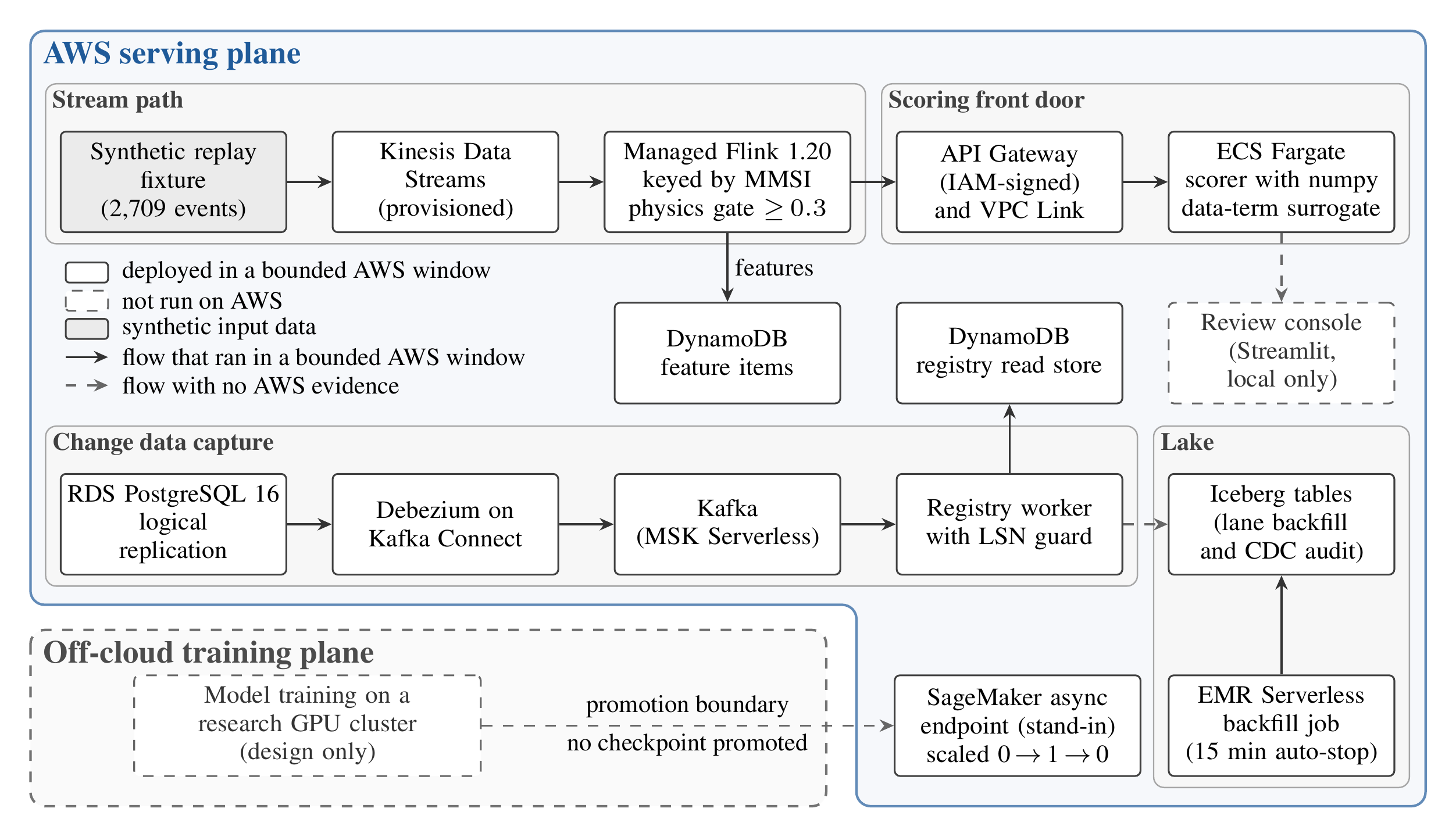
Figure 1. Harbormaster separates an off-cloud training plane from an AWS serving plane. Training on a research GPU cluster is design only, and no trained checkpoint crossed the promotion boundary. Solid boxes are components that were deployed in a bounded AWS window, and solid arrows are flows that ran in a bounded AWS window. Dashed boxes did not run on AWS, and dashed arrows mark flows with no AWS evidence. The ECS task sets no endpoint, so the scorer took its data term from a numpy surrogate on AWS, and the figure draws no arrow between the scorer and the endpoint.
Abstract
Ships broadcast their positions through the Automatic Identification System (AIS), and those reports can be false or missing. An operator who acts on an anomaly alert needs that alert to be attributable, reviewable, and recoverable after a failure. This paper describes Harbormaster, a production-shaped system on AWS that follows three rules. Physics checks run on every report before any learned model runs. The DynamoDB read store is an idempotent projection of PostgreSQL, and a guard on the log sequence number (LSN) of each change protects every write to it. A candidate model must pass a holdout gate and a shadow comparison before a canary gives it traffic, and a burn-rate check guards each canary step. The paper proves that replaying any prefix or suffix of the change log leaves each projected key at the value of its highest applied LSN. It also names the effects that this result does not cover, such as repeated cache invalidations and repeated audit rows. In a bounded AWS window, a one-hour soak returned 35,999 HTTP 200 responses to 36,000 requests, with a 95th-percentile (p95) client latency of 142.751 ms. In a separate bounded AWS run of 900 s, the stream path received a burst of 400 records/s, and its consumer lag later drained to zero. Every number in the paper carries a label that says where it was measured, and the paper lists the parts of the design that were never built.
System overview
Figure 1, at the top of this page, shows the two planes of Harbormaster. The training plane belongs on an off-cloud research GPU cluster, and the paper treats it as design only. The serving plane runs on AWS, and its parts ran in bounded windows. No trained checkpoint was promoted into AWS serving, so the model endpoint served a labeled demo stand-in image.
The design has five workflows, and each one has its own trigger. Workflow 1 checks each incoming vessel report, and Workflow 2 saves an analyst's review label. Workflow 3 carries committed registry changes into the serving copies, and Workflow 4 builds shipping-lane context from historical batches. In the design, Workflow 5 submits a separate model job to an asynchronous endpoint, and its job service, dispatch worker, and result collector are not built. The ingestor replays only a synthetic replay fixture of 2,709 events for 8 vessels over 6 hours, and no real-time AIS source was connected.
Position reports and database changes travel on separate brokers. Provisioned Amazon Kinesis carries position reports, and Managed Flink 1.20 consumes them with state keyed by the vessel's MMSI (Maritime Mobile Service Identity). Kafka carries Debezium change events. The Flink job keeps the last five fixes for each vessel and applies the physics gate to each report. For each report that passes, it writes a feature item to DynamoDB and posts a signed request to the scorer.
The scorer is a FastAPI service on ECS Fargate, and it is the entry point for every scoring request. Requests reach it through an API Gateway HTTP API with IAM authorization and a VPC Link, so the path has no standing load balancer. The ECS task on AWS set no model endpoint, so the data term \(P_{\mathrm{data}}\) came from a numpy surrogate there. The Streamlit review console ran only locally.
Physics-first scoring
The scorer uses physics as its first source of evidence. Each rule is a closed-form function of the reported fixes and the reference data, so an analyst can recompute any score from the constants in the public code.
The stream gate
For consecutive fixes \(A\) and \(B\), the system computes the haversine distance \(d_{AB}\) and the speed \(v_{\mathrm{req}}\) that the move requires. The plausibility \(p_{\mathrm{phys}}\) equals 1 when a vessel at the speed cap could make the move, and it falls as the required speed rises.
The speed cap is \(v_{\max} = 25\) knots, which is 12.861 m/s, and the constant \(\epsilon\) is \(10^{-6}\), in seconds inside the first maximum and in m/s inside the second. The Flink job forwards a report to the scorer only when \(p_{\mathrm{phys}} \ge 0.3\).
This gate delays the scoring of fast jumps, and it can also drop them. It drops every report whose required speed from the previous stored fix exceeds \(v_{\max}/0.3\), which is about 83 knots. The Flink job still adds the dropped fix to the vessel's five-fix history, so a jump between about 83 and 300 knots is scored late, when a later report passes the gate. The jump goes unscored when the vessel's next four reports also fail the gate or never arrive. A jump above 12 \(v_{\max}\), which is 300 knots, makes every later request that still carries both of its fixes fail with HTTP 422.
The space-time prism
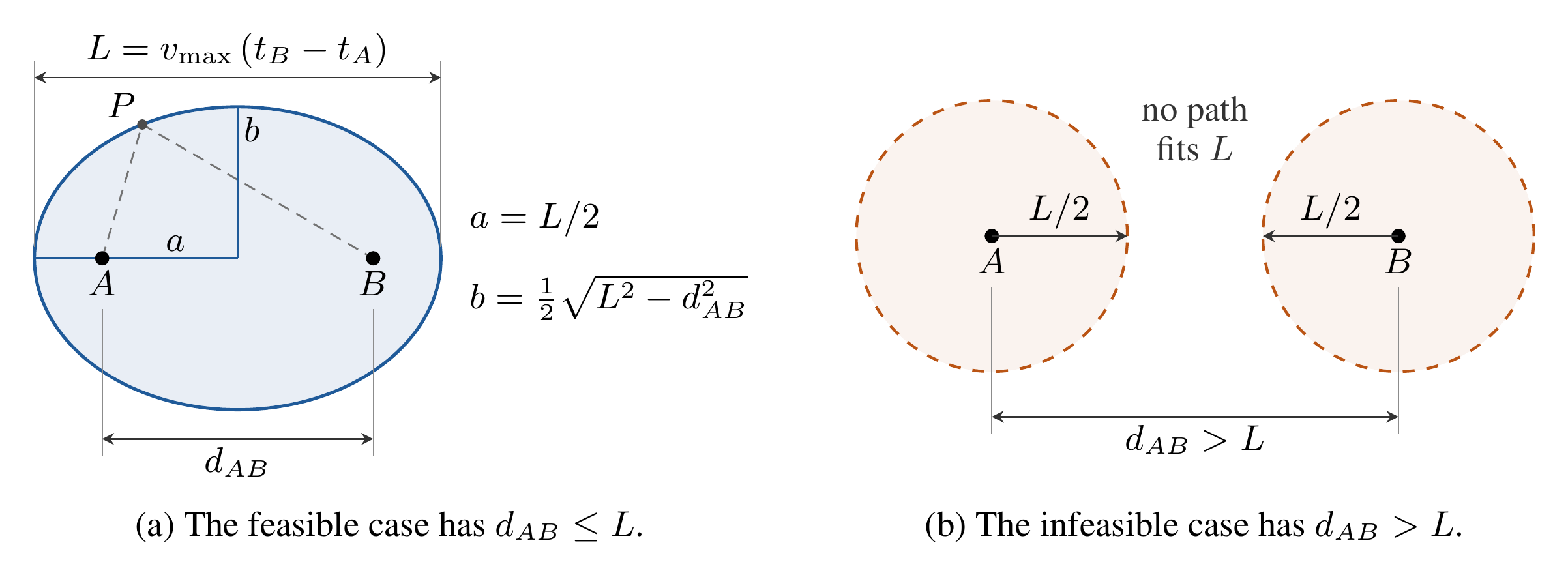
Figure 2. The space-time prism tests whether one vessel could have moved between two fixes at the speed cap. Fixes \(A\) and \(B\) lie a distance \(d_{AB}\) apart, and the reach length is \(L = v_{\max}(t_B - t_A)\), where the code sets \(v_{\max}\) to 25 knots. (a) When \(d_{AB} \le L\), the feasible positions fill an ellipse with foci \(A\) and \(B\), semi-major axis \(a = L/2\), and semi-minor axis \(b = \tfrac{1}{2}\sqrt{L^2 - d_{AB}^2}\). A point \(P\) on the boundary satisfies \(|AP| + |PB| = L\). (b) When \(d_{AB} > L\), the reach disks of radius \(L/2\) around \(A\) and \(B\) do not meet at the midpoint time, so no path fits within \(L\).
The space-time prism is the set of places that a vessel could occupy between two fixes if it never exceeded \(v_{\max}\). Its footprint on the map is an ellipse with foci at \(A\) and \(B\), and the reach length \(L\) sets the size of that ellipse.
\[ L = v_{\max}\,(t_B - t_A) \]\[ \text{feasible} \iff d_{AB} - \delta \le L \]
\[ a = \tfrac{1}{2}L, \qquad b = \tfrac{1}{2}\sqrt{\max\!\big(0,\,L^2 - d_{AB}^2\big)} \]
The code allows a tolerance of \(\delta = 10^{-6}\) m. On the single-vessel scoring path, the scorer computes this prism for the latest pair of fixes, and the fused score does not read the result. The feasibility test for that pair matches the speed test \(v_{\mathrm{req}} \le v_{\max}\) up to \(\delta\), so the speed detector already scores the same condition. The prism geometry matters inside the gap detector, which merges candidate gaps whose prism bounding rectangles overlap.
The abnormal gap measure
A silence longer than the 600 s coverage threshold opens a candidate gap. The gap detector follows earlier work on abnormal gap detection, and Harbormaster keeps the name abnormal gap measure (AGM) for its own formula. The formula blends kinematic implausibility with a data term.
Here \(d\) is the gap distance in meters, \(\Delta t\) is the gap duration in seconds, and clip limits a value to the range from 0 to 1. The detector merges candidate gaps whose prisms overlap, and the scorer keeps the group with the largest AGM. The \(P_{\mathrm{data}}\) formula is a numpy surrogate, and on AWS the term came from that surrogate. The target design replaces it with a diffusion model trained on the off-cloud cluster.
Fusion and review
The scorer fuses the severities \(s_i\) of all reasons with a noisy-OR rule, which treats the reasons as separate pieces of evidence. One strong reason can therefore raise the score close to 1 by itself.
\[ S = 1 - \prod_{i}(1 - s_i) \]\[ c = 1 - 2\min(S,\,1 - S) \]\[ \text{review} \iff c < 0.7 \ \lor\ S \ge 0.6 \]
The confidence \(c\) is 1 at the ends of the score range and 0 at \(S = 0.5\). The confidence depends only on \(S\), so the rule sends a case to review exactly when \(S > 0.15\). The analyst's label is stored next to the case, and it never overwrites the automated score.
The planner chooses detectors from the length of the history, and it uses no language model. It always runs the corridor detector. It adds the prism, speed, and validate steps when the history holds at least one prior fix, and it adds the gap detector when the history holds at least three.
Replay-safe change data capture
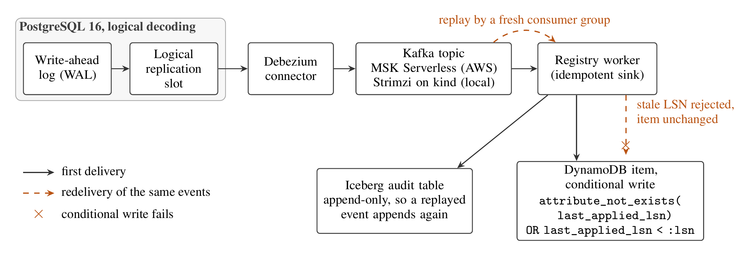
Figure 3. The change data capture (CDC) path copies PostgreSQL 16 changes into DynamoDB. Debezium reads the write-ahead log through a logical replication slot and publishes change events to Kafka. Kafka ran as Amazon MSK Serverless in the bounded AWS window and as Strimzi on kind locally. The registry worker writes each item with the conditional write shown, so the write succeeds only when the item has no applied LSN or holds an older one. A replayed event with a stale LSN fails that condition and leaves the item unchanged. The Iceberg audit table appends every delivered event, so its rows can repeat after a redelivery. No AWS record shows the audit append, so Figure 1 draws that edge dashed.
PostgreSQL 16 on RDS holds the authoritative vessel, watchlist, and sanctions tables, and every other copy of that data is derived. Debezium runs inside Kafka Connect and reads committed changes through logical replication. Kafka delivers each change event at least once, so a consumer restart or a replay can deliver the same event again. For each event, a registry worker attempts a conditional write to the DynamoDB read store, removes the stale Redis cache entry, and appends a row to an Iceberg audit table.
The worker applies every event in a batch, flushes every sink, and only then commits its Kafka offsets. When a sink fails, the offsets stay uncommitted, and Kafka redelivers the batch. A source delete becomes a soft-delete item that the worker writes at the delete's own LSN.
The LSN-guarded write
Each item in the read store keeps the log sequence number (LSN) of the change that last wrote it. The worker writes with a DynamoDB conditional put. The condition compares the stored LSN \(\ell^\star(k)\) of key \(k\) with the incoming LSN \(\ell\).
Here \(\bot\) means that the item has no stored LSN yet. A rejected write signals a stale or duplicate delivery, so the worker records the event as not applied and raises no error. The worker applies rows from Debezium's initial snapshot at \(\ell = 0\). A snapshot row therefore applies only to an empty key, and every streamed change outranks it.
The replay proposition, in words
The paper proves one proposition about replay into a projection that starts empty, and the proposition makes four assumptions. For each key, an LSN identifies at most one value. The check and the write happen atomically for each item. Each accepted write replaces the whole item, and every delivered event maps to a valid item key.
Under these assumptions, the worker can process any finite sequence of deliveries drawn from the change log, in any order and with any repetition. Afterward, each key that appears in the sequence holds the value of its highest-LSN event, and every other key stays empty. Replaying any prefix or suffix of the log after a full pass therefore leaves each projected key at the value of its highest applied LSN. The proof uses induction on the length of the delivery sequence.
This result also needs a log that holds every committed change. That condition fails if the replication slot is dropped or invalidated. A re-snapshot after such a loss cannot repair a key that already holds a streamed LSN, because the guard rejects snapshot rows at LSN zero.
What the guard does not cover
The proposition covers one sink and one key at a time, and the paper claims nothing stronger. Redis invalidations can repeat after a redelivery. The Iceberg audit table appends every delivered event, so a redelivered batch appends its rows again. The worker buffers audit rows until the batch flush, so a crash in the middle of a batch can lose those rows. The worker also skips a content error, which is an event that no key mapping can apply. It audits that event as not applied and commits past it, so redelivery never repairs that key.
A reader can also see one key updated before another, because the guard orders changes per key only. The paper therefore describes this path as an idempotent, LSN-guarded projection. It does not claim that each change takes effect once across every destination.
Slot-lag monitoring
A logical replication slot makes PostgreSQL retain write-ahead log (WAL) until the consumer confirms it, so a stalled consumer makes the database hold disk. The monitor measures slot lag in bytes, and a CloudWatch alarm fires at 200 MiB.
\[ \Delta_{\mathrm{slot}}(t) = \mathrm{LSN}_{\mathrm{current}}(t) - \mathrm{LSN}_{\mathrm{confirmed}}(t) \]\[ \text{alarm at minute } t \iff \min_{j \in \{0,1,2\}} M_{t-j} \ge \theta_{\mathrm{slot}} \]
Here \(M_t\) is the largest slot lag that the monitor publishes in one-minute period \(t\), so the alarm needs three consecutive periods at or above the threshold. The threshold \(\theta_{\mathrm{slot}}\) is 209,715,200 bytes. A slot can also fall behind while its captured tables are quiet, and a Debezium heartbeat query that upserts one row handles that case.
Evidence-gated promotion
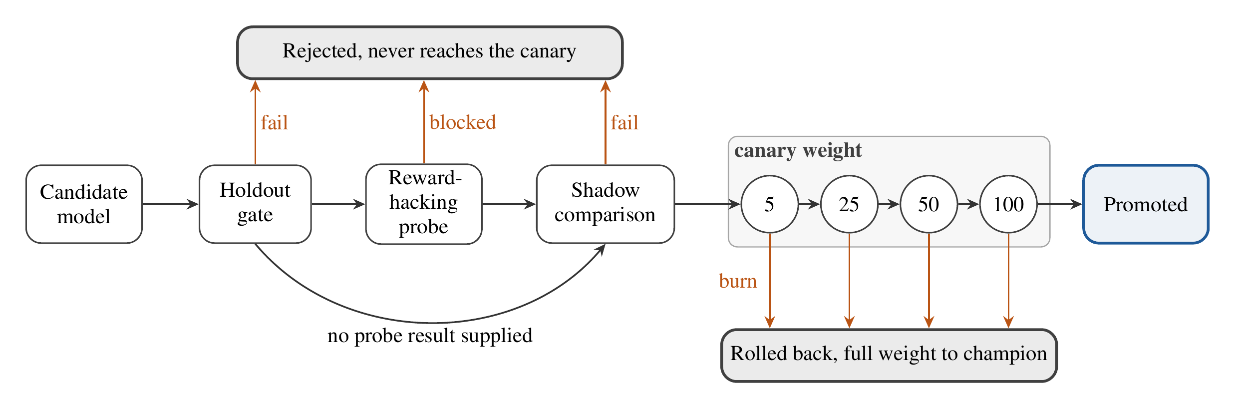
Figure 4. The promotion ladder moves a candidate model through up to four checks. Black edges move the candidate forward, and orange edges end the promotion. The candidate must pass the holdout gate, then the reward-hacking probe when a probe result is supplied, and then the shadow comparison. Every gate has a reject edge, and a rejected candidate never reaches the canary. The canary advances through weights 5, 25, 50, and 100 while the burn rate stays healthy, and a burn at any step returns the full weight to the champion. The gate results reported in the paper come from synthetic drills. The live asynchronous endpoint has one variant, so the canary moved no traffic on AWS.
A candidate model reaches traffic only through the ladder in Figure 4. The ladder has up to four steps, which are a holdout gate, a reward-hacking probe, a shadow comparison, and a weighted canary. A failure at any step stops the candidate. The probe runs only when the caller supplies a probe result, so supervised retraining candidates skip it.
Holdout gate
The holdout gate requires an AUC of at least 0.85, a mean continuous ranked probability score (CRPS) of at most 1.0, and a calibration ratio inside \([0.8, 1.2]\). The model predicts a Gaussian \(\mathcal{N}(\mu, \sigma^2)\) for each observation \(y\), and CRPS has a closed form for that case.
\[ \rho = \frac{\overline{e^2}}{\overline{\sigma^2}}, \qquad e = y - \mu \]
Here \(\Phi\) and \(\varphi\) are the standard normal distribution and density functions, and a bar denotes a mean over the holdout set. Every threshold must pass, so a strong AUC cannot make up for poor calibration.
Reward-hacking probe
The probe compares a preference-tuned candidate with the baseline on a held-out set. The rule uses the mean total reward \(\bar R\), the rate \(u\) of structural-constraint violations, and the mean structural term \(\bar s\).
The rule blocks a candidate whose reward rises while its physical consistency gets worse. The second clause catches a candidate that keeps the same number of violations and makes each one more severe.
Shadow comparison
The shadow step scores the same \(N\) inputs with the champion and the candidate. It passes when the mean absolute score difference is at most a limit \(\delta_{\mathrm{sh}}\) that the caller sets, and the drills set it to 0.05.
The canary moves the candidate through the weights 5, 25, 50, and 100. At each weight, a burn-rate check reads the score-success service level objective (SLO). The burn rate \(B_W\) of a window \(W\) divides its observed bad ratio by the allowed error fraction \(1 - T\), where \(T\) is the SLO target.
A burn rate above 14.4 over 1 h and 5 min pages, and a burn rate above 6 over 6 h and 30 min also pages. A burn rate above 3 over 1 day and 2 h raises a warning. A page at any canary weight reverts the full weight to the champion in one action, and a warning does not revert.
The feedback loop ends at preference data. A builder turns analyst labels of incorrect into offline preference records, and no code path retrains a model from them. No reinforcement-learning fine-tune ran, so no real candidate has reached the probe. The live endpoint allows one variant, so the canary is traffic-inert there, and the shadow and canary results on this page come from synthetic drills.
Scale-to-zero serving
In the design, the heavier model runs behind a SageMaker asynchronous inference endpoint. The endpoint holds a request queue, so it can accept a request while it has no instance and serve that request after it wakes. Its autoscaling target allows between zero and one instance, and two policies share that target.
A target-tracking policy steers the metric ApproximateBacklogSizePerInstance toward a setpoint of 5. When the backlog empties, it scales the endpoint in to zero instances. Target tracking cannot see the move from zero instances, so a separate step policy handles it. The step policy sets the capacity to exactly 1 when the average \(\bar H_k\) of HasBacklogWithoutCapacity is at least 1 in two consecutive 60 s periods, and its cooldown is 60 s.
Two dimension bugs
Both policies had a bug in their CloudWatch metric dimensions. An AI audit session compared the SageMaker Terraform with AWS's own canonical examples and returned 19 numbered findings. Its first finding, which the public repository's incident log records as P25, was that the target-tracking metric specification lacked the EndpointName dimension. SageMaker publishes the metric under that dimension, so the policy's alarms queried a series that does not exist, and scale-in to zero could never fire. The audit found the gap from the code alone, before any live symptom appeared.
In a bounded AWS window, a live check of that fix exposed a second bug, P26. The wake alarm carried an extra VariantName dimension, and SageMaker does not publish HasBacklogWithoutCapacity under it. The alarm received no datapoints for more than 15 minutes while a real backlog waited, so the endpoint would never have woken from zero. P26 is not one of the 19 audit findings. Both bugs left every resource present and every apply clean, and neither bug raised an error.
Evidence on the endpoint
In a bounded AWS window, a controlled drill woke the endpoint from zero instances. The backlog alarm fired, capacity moved to one, and the same request returned a score. The endpoint then returned to zero instances. The record gives no wake time, so the paper reports none. The endpoint served a labeled demo stand-in image.
A KEDA ScaledObject on EKS gives a second scale-from-zero path for a serving deployment. This path ran once in a bounded AWS window and was then torn down, and ECS stayed the entry point.
Evaluation
Every result names where it was measured. BOUNDED-AWS-WINDOW marks a measurement on real AWS resources during one attended, time-boxed window, and its evidence is private. LOCAL marks a run on a local machine or a local stack. SYNTHETIC-DRILL marks a deterministic drill that runs real project code on synthetic inputs without any infrastructure. PUBLIC-REPO marks a result that the public repository states or reproduces. No experiment measures detection accuracy.
Table 1. Each measured result appears with its scope. A reader can rerun the public test suite, the local CDC tests, and the public scripts for the skew, canary, and slot drills. The soak row carries PUBLIC-REPO because the public README restates it, and it cannot be rerun. The AWS rows come from bounded windows whose evidence is private.
Result
Value
Scope
SageMaker wake from zero
0 to 1 to 0 instances, no wake time recorded
BOUNDED-AWS-WINDOW
Stream run load
34,123 records in 900 s, 5 records/s with a 400 records/s burst from 60 to 135 s
BOUNDED-AWS-WINDOW
Backpressure, source and key-by vertex
0.927 in the burst window, 0.998 after it, below 0.1 at about 694 s
BOUNDED-AWS-WINDOW
Lag, one-minute maxima
139 s for Kinesis and for Flink, then 0
BOUNDED-AWS-WINDOW
Scale request to first HTTP 200, KEDA on EKS
1.89 s
BOUNDED-AWS-WINDOW
One-hour soak outcomes
35,999 of 36,000 HTTP 200, one 503
BOUNDED-AWS-WINDOW, PUBLIC-REPO
Soak latency, p95 and p99
client 142.751 and 240.283 ms, server 7.048 and 9.348 ms
BOUNDED-AWS-WINDOW
CDC acceptance on MSK Serverless
drills A to E passed, replay hash unchanged
BOUNDED-AWS-WINDOW
Local CDC end-to-end tests
5 passed in 36.41 s on a fresh stack
LOCAL, PUBLIC-REPO
Insert to read store
0.57 s against a 5 s target
LOCAL
Slot growth and drain
74,035,000 bytes, then 0
LOCAL
Stale event after a newer one
guarded severity held at 0.95
SYNTHETIC-DRILL
Candidate with serving skew
holdout passed, shadow 0.6056 against 0.05
SYNTHETIC-DRILL
Canary with planted regression
reverted at weight 25
SYNTHETIC-DRILL
Scoring kernel latency
p95 0.6109 ms on one thread
LOCAL
AI audit of SageMaker Terraform
19 findings in four groups
LOCAL
Public snapshot test suite
821 passed, 12 skipped, 83.72% coverage
PUBLIC-REPO
Private regression suite
1,633 passed, 21 skipped
LOCAL
Stream run under load
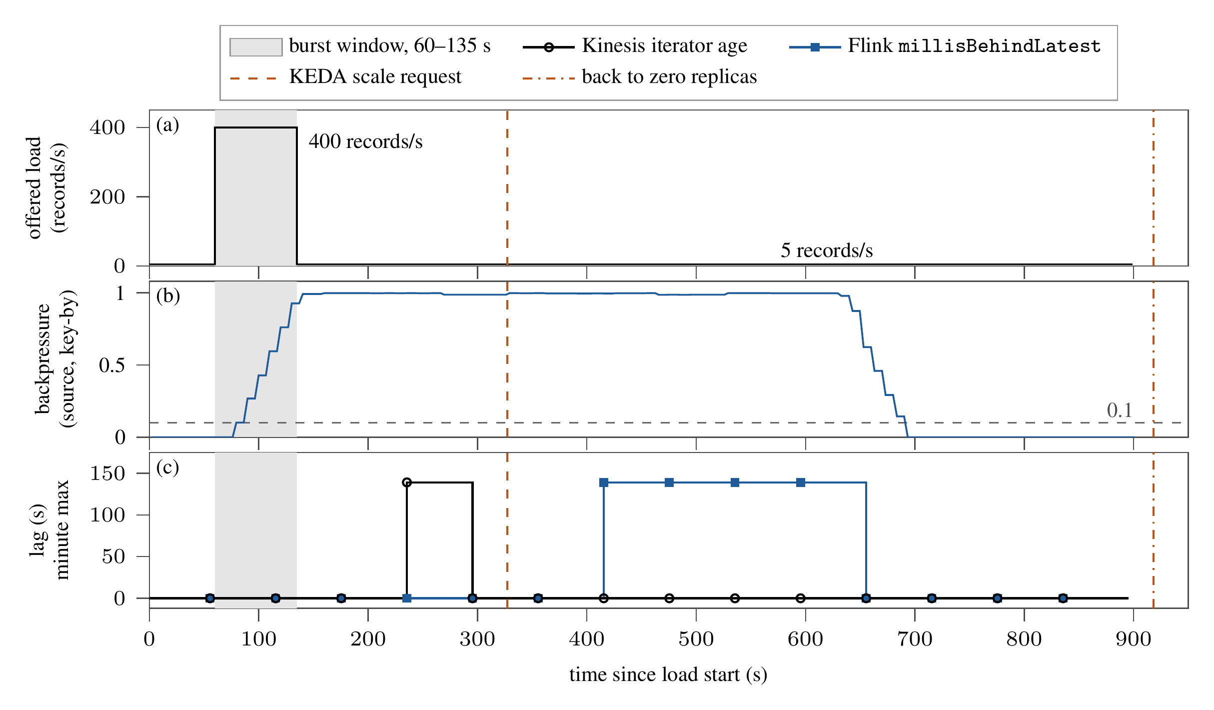
Figure 5. The stream run shows offered load, backpressure, and lag from one bounded AWS window. (a) The load generator cycled the synthetic replay fixture into provisioned Kinesis at 5 records/s, with a burst of 400 records/s from 60 to 135 s. Managed Flink consumed the stream. The run measured the pipeline under load and did not measure detection quality. (b) Backpressure on the source and key-by vertex reached 0.927 inside the gray burst window and 0.998 after it. It dropped to the dashed 0.1 line or below near 694 s. (c) CloudWatch reports lag at one-minute resolution, so each step holds a per-minute maximum. Both series peaked at a lag of 139 s and then drained to 0. The vertical lines mark a separate KEDA on EKS scale-from-zero test in the same window. The dashed line marks the scale request at 327.37 s. The first HTTP 200 came 1.89 s later, at 329.26 s, so the figure does not draw it as a separate line. The deployment returned to zero replicas at 918.24 s.
A producer sent 34,123 records into provisioned Kinesis over a 900 s run. The load held 5 records/s, except for a burst of 400 records/s from 60 s to 135 s. Backpressure on the source and key-by vertex reached 0.927 inside the burst window. It kept rising after the burst ended and first reached 0.998 about 160 s after the load started. It cleared below 0.1 at about 694 s.
Kinesis iterator age and Flink millisBehindLatest each peaked at 139,000 ms in one-minute buckets, and both series then drained to 0. The run measured the pipeline under load, and it did not measure detection quality.
One-hour soak through the ECS entry point
The soak tested serving capacity in a bounded AWS window. Each request passed through the IAM-signed API Gateway route and the VPC Link to the ECS service. One 3,600 s trial offered 10 requests per second with open-loop arrivals and no retries. It returned 35,999 HTTP 200 responses and one HTTP 503, for a success ratio of 0.99997 against a 0.999 gate.
Client latency had a p95 of 142.751 ms and a p99 of 240.283 ms. Server latency had a p95 of 7.048 ms and a p99 of 9.348 ms. The soak repeated one fixed request whose history held one fix. The planner therefore ran the corridor, prism, speed, and validate steps, and it never ran the gap detector or the \(P_{\mathrm{data}}\) term. The soak also started prewarmed after a successful preflight, so it supports no cold-start claim. It measures serving capacity, and it measures no detection quality.
CDC and gate drills
A bounded AWS window ran the CDC path on an MSK Serverless cluster, and five drills passed. In one drill, a replay with a fresh consumer group read 3 tombstones, and the LSN guard rejected 3 change events. The 3 DynamoDB items and their content hash did not change.
In a local slot drill, a logical slot with no consumer grew from 6,926,136 to 74,035,000 bytes, and draining the slot returned the lag to 0. In a synthetic duplicate drill, a stale event made the unguarded sink regress the severity from 0.95 to 0.9, and the guarded sink kept 0.95.
Two synthetic drills run the real gate code with a synthetic toy scorer and synthetic AIS-shaped inputs. In the skew drill, a candidate had a bug in its online feature encoding. The holdout gate passed it, and the shadow comparison failed it with a mean absolute difference of 0.6056 against the 0.05 limit. The drill builds its holdout data so that the candidate passes, so the holdout result does not measure a model. In the canary drill, the canary advanced to weight 5 and met a planted regression at weight 25. The rollback step then returned the full weight to the champion. The drill injects the burn check, so it tests the revert path and does not exercise the burn-rate formula.
What is not built
The paper claims none of the following as running.
Candidate V3, a model candidate, is not deployed. The AWS endpoint served only a labeled demo stand-in image, so no trained model produced a served score.
No reinforcement-learning fine-tune ran, and the feedback loop ends at offline preference data.
Distributed tracing was never built, and the paper reports no drift monitoring on AWS.
CDC on AWS ran only in bounded acceptance windows. The canary is single-variant and traffic-inert on the live endpoint.
The stream carried synthetic load, and the ingestor replays only a synthetic fixture. The Flink job has no event-time windows or watermarks, and its gate scores some fast jumps late or drops them.
The lane release publisher is an assumed integration, and the review console ran only locally.
The Workflow 5 job service, dispatch worker, and result collector are not built.
The paper also claims no detection accuracy, no false-alert rate, and no result on real labeled cases. It claims no SLO, no cold-start time, and no SageMaker wake time.